CO2 pre-salt phase behavior across applicable models

This report compares every native torch-flash equation of state that covers the CO2/n-hexadecane, CO2/n-hexadecane/methane, and CO2/n-hexadecane/methane/phenanthrene systems measured by Simoncelli et al., Fluid Phase Equilibria 515 (2020) 112574, doi:10.1016/j.fluid.2020.112574. The study contains all 157 observations from Tables 7–9: 37 liquid to liquid-liquid (L-LL), 21 liquid-liquid to vapor-liquid-liquid (LL-VLL), and 99 liquid to vapor-liquid (L-VL) transitions.

The reported instrument uncertainties are 0.1 K and 0.05 MPa. They do not represent composition, visual-transition, or model-form uncertainty.

Model and evidence scope

SRK, PR76, PR78, and E-PPR78-2022 cover every component. The conventional cubics use the paper's Table 3 pure-component constants and quadratic mixing. Their unfitted baselines set every attraction and covolume interaction to zero. E-PPR78 uses the global group-contribution correlation of Jaubert et al., doi:10.1016/j.fluid.2022.113456, and remains predictive.

GERG-2008 and EOS-CG-2021 omit n-hexadecane and phenanthrene. The bundled CPA and activity/Huron-Vidal parameter sets do not cover the complete component set. A consistent volume translation is not treated as a separate VLE model because it leaves phase-equilibrium fugacity equalities unchanged.

Unfitted and predictive comparisons are experimental validation. Post-fit agreement on the 136 two-phase observations is calibration evidence because those observations enter the objective. The 21 LL-VLL states remain experimental validation after fitting because they are excluded from parameter estimation.

Three Table 7 labels give CO2 mole fractions 0.9838, 0.9370, and 0.9090, whereas Table 2 and Figure 4 identify the same mixtures as 0.9839, 0.9369, and 0.9098. The repeated Table 2/Figure 4 identities are used here.

Full phase-envelope calculation

Each curve is a boundary between equilibrium phase regions on a fixed-composition \(P\)-\(T\) grid, not a polyline through transition observations. flash_grid evaluates an 80 by 80 grid over 250–750 K and 0.2–80 MPa. identify_grid_phases labels the converged regions, and refine_flash_grid_phase_boundaries re-flashes label-changing edges with four batched bisection passes before reconnecting the boundary crossings.

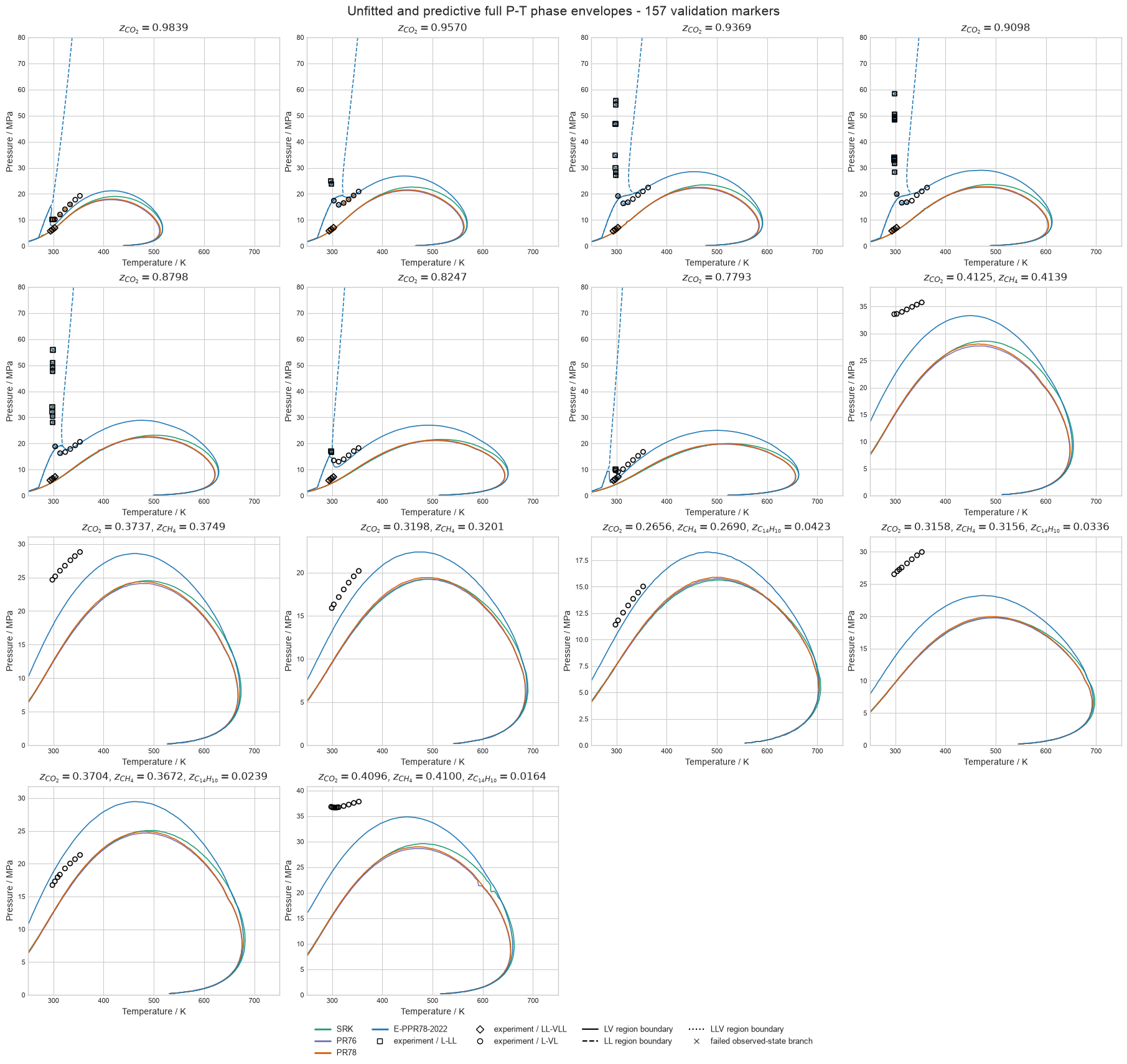
Diamonds, squares, and circles are respectively the experimental LL-VLL, L-LL, and L-VL observations from Simoncelli et al. Every one of the 157 reported transition states is plotted; the continuous curves are torch-flash calculations and are not lines fitted through the markers.

Successful refinement passes target brackets no wider than approximately 0.40 K or 0.063 MPa. If a midpoint flash fails, the edge bracket is left unchanged rather than assigning an unsupported phase label. The QA table therefore reports both failed midpoint states and the largest retained bracket.

Phase-grid QA	Unfitted/predictive	Fitted conventional
Model-composition grids	56	42
Converged cells / total	358,400 / 358,400	268,797 / 268,800
Maximum fugacity residual	\(1.00\times10^{-8}\)	\(1.00\times10^{-8}\)
Maximum material-balance residual	\(1.49\times10^{-14}\)	\(1.41\times10^{-11}\)
High-temperature closure inside grid	56 / 56	42 / 42
Multiphase region below 80 MPa	49 / 56	22 / 42
Refined crossing edges	12,008	10,040
Failed midpoint states	9	34
Maximum retained temperature bracket / K	0.791	3.165
Maximum retained pressure bracket / MPa	1.010	1.010

Curves beyond the measured 294–363 K interval are fluid-model extrapolations. Solid phases are outside the calculation, so low-temperature fluid boundaries can be metastable. Boundaries that reach 80 MPa are domain-truncated rather than reported as physically closed.

Part I: unfitted and predictive results

Coverage retains every observation in the denominator. AARD and RMSE use only residual-converged, physically separated branches and must be read together with coverage.

Model	Converged / 157	Coverage / %	AARD / %	RMSE / MPa
SRK, zero interactions	96	61.15	43.91	11.25
PR76, zero interactions	90	57.32	42.23	11.26
PR78, zero interactions	91	57.96	42.39	11.21
E-PPR78-2022, predictive	109	69.43	15.31	5.64

Model	Transition	Converged / total	Coverage / %	AARD / %	RMSE / MPa	Bias / MPa
SRK	L-LL	3 / 37	8.11	62.30	8.33	-7.78
SRK	L-VL	93 / 99	93.94	43.31	11.33	-10.02
SRK	LL-VLL	0 / 21	0.00	—	—	—
PR76	L-LL	0 / 37	0.00	—	—	—
PR76	L-VL	90 / 99	90.91	42.23	11.26	-9.88
PR76	LL-VLL	0 / 21	0.00	—	—	—
PR78	L-LL	0 / 37	0.00	—	—	—
PR78	L-VL	91 / 99	91.92	42.39	11.21	-9.88
PR78	LL-VLL	0 / 21	0.00	—	—	—
E-PPR78-2022	L-LL	2 / 37	5.41	25.33	2.59	-2.59
E-PPR78-2022	L-VL	89 / 99	89.90	17.69	6.23	-3.79
E-PPR78-2022	LL-VLL	18 / 21	85.71	2.44	0.165	-0.155

The zero-interaction results are model-form baselines, not recommended reservoir-fluid parameterizations.

Part II: simultaneous conventional-cubic calibration

One differentiable full-batch objective contains all 136 two-phase observations simultaneously. At every optimizer evaluation, all observations are evaluated at their measured temperature, pressure, and overall composition. The objective uses the observed-state fugacity mismatch with physically separated latent incipient compositions, plus a dimensionless quadratic parameter-displacement penalty of 10 around the published Table 4 interaction vector.

The seven shared parameters are six symmetric attraction interactions and the CO2/n-hexadecane covolume interaction. Attraction interactions are bounded to \([-0.20, 0.35]\), and the covolume interaction to \([-0.15, 0.15]\), through a differentiable bounded transform.

PyTorch L-BFGS uses a strong-Wolfe line search, an iteration budget of 2,000, and 30 evaluated losses of no improvement as the early-stop patience. All three fits met the numerical tolerance rather than exhausting the budget or stopping on patience.

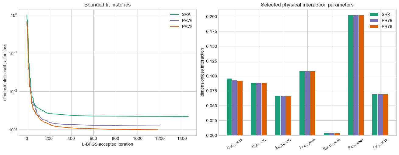
Model	Accepted iterations	Initial loss	Selected iteration	Selected loss	Fit and sensitivity / s
SRK	1,457	1.012422	1,457	0.002200	43.51
PR76	1,199	0.677006	1,199	0.001243	39.95
PR78	1,179	0.650156	1,178	0.000992	40.10

Interaction	SRK	PR76	PR78
\(k_{\mathrm{CO2,nC16}}\)	0.095644	0.092781	0.091973
\(k_{\mathrm{CO2,CH4}}\)	0.088373	0.088372	0.088370
\(k_{\mathrm{nC16,CH4}}\)	0.066277	0.066253	0.066224
\(k_{\mathrm{CO2,phen}}\)	0.108004	0.108010	0.108003
\(k_{\mathrm{nC16,phen}}\)	0.003897	0.003881	0.003891
\(k_{\mathrm{CH4,phen}}\)	0.202510	0.202513	0.202510
\(l_{\mathrm{CO2,nC16}}\)	0.068889	0.068837	0.068872

The local sensitivity audit contains 361 finite residual rows for each model. All seven parameter directions have nonzero local singular values.

Model	Local rank / 7	Largest singular value	Smallest singular value	Condition number
SRK	7	75.07	1.833	40.95
PR76	7	82.18	1.881	43.70
PR78	7	82.99	1.816	45.70

Three-phase recovery

The LL-VLL states are binary three-phase invariants: fixed temperature gives one equilibrium pressure and three phase compositions. Generic starts that place one liquid near zero CO2 converge to a merged algebraic branch for this CO2-rich system. The evaluator now includes physically separated, all-CO2-rich invariant starts.

The fast path solves compatible invariant states in one PyTorch Newton batch. For fitted conventional cubics, the selected branch is then polished or recovered with the vectorized exact-Hessian trust-region method. The restricted-step method follows Petitfrere and Nichita, Fluid Phase Equilibria 362 (2014) 51–68, doi:10.1016/j.fluid.2013.08.039. Only the tiny dense Moré-Sorensen spectral subproblem is handled per state; thermodynamic residual, gradient, and Hessian evaluations remain batched.

All 21 post-fit LL-VLL states converge for SRK, PR76, and PR78:

Model	Converged / 21	AARD / %	RMSE / MPa	Bias / MPa	Maximum fugacity residual
SRK	21	1.751	0.129	-0.114	\(2.86\times10^{-11}\)
PR76	21	2.098	0.149	-0.136	\(1.51\times10^{-10}\)
PR78	21	1.982	0.142	-0.128	\(1.49\times10^{-11}\)

These are validation results because the LL-VLL observations were not used by the fit.

Fitted results

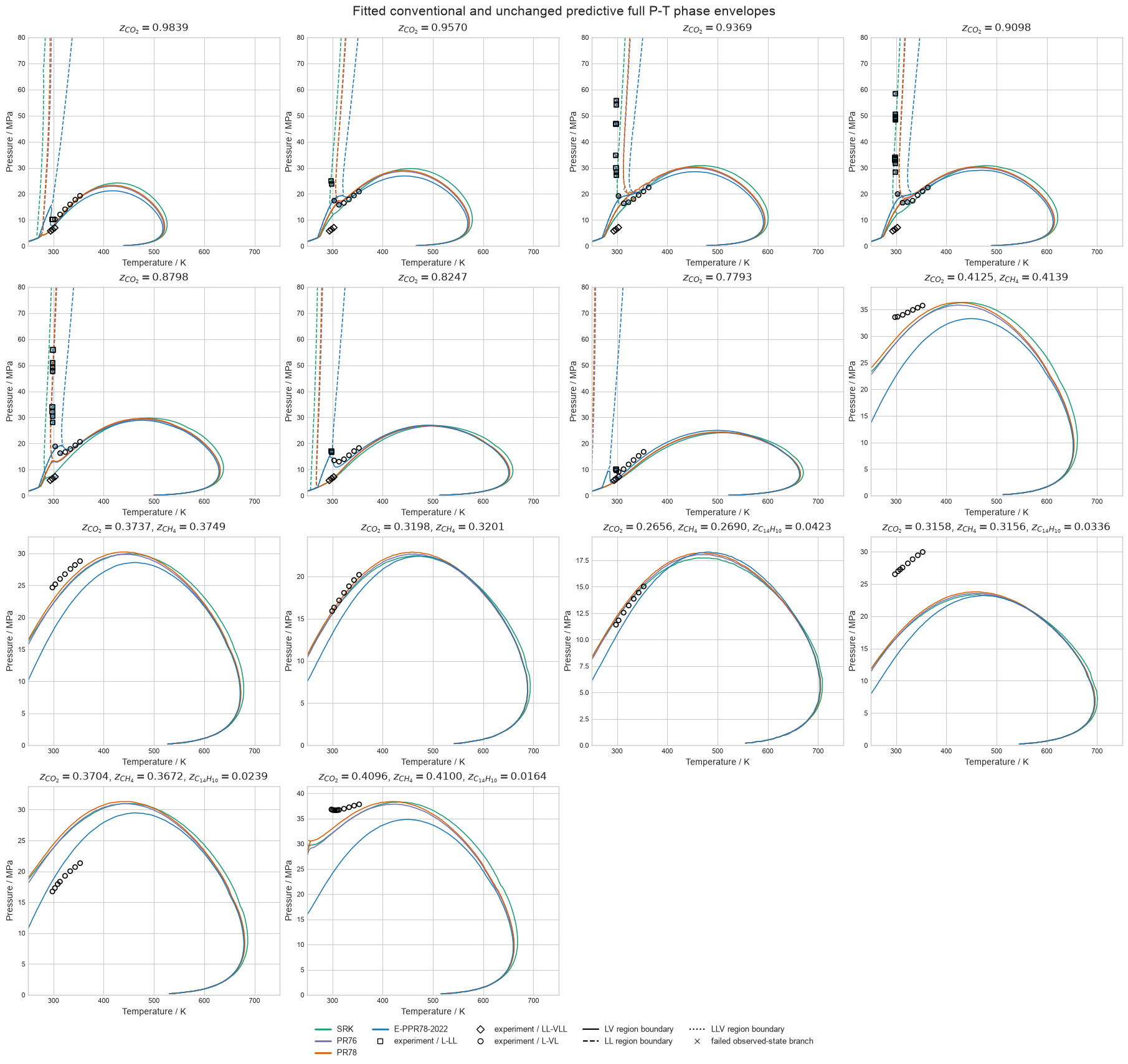
The same 157 Simoncelli et al. experimental markers are retained so that before/after changes can be compared against identical observations. The continuous E-PPR78 curve is unchanged because that predictive model was not calibrated.

Model	Status	Converged / 157	Coverage / %	AARD / %	RMSE / MPa
SRK	fitted	134	85.35	14.22	4.72
PR76	fitted	127	80.89	13.92	4.46
PR78	fitted	126	80.25	13.82	4.56
E-PPR78-2022	predictive, unchanged	109	69.43	15.31	5.64

Model	Transition	Converged / total	Coverage / %	AARD / %	RMSE / MPa	Bias / MPa
SRK	L-LL	15 / 37	40.54	22.49	8.34	-0.76
SRK	L-VL	98 / 99	98.99	15.63	4.45	-2.11
SRK	LL-VLL	21 / 21	100.00	1.75	0.129	-0.114
PR76	L-LL	10 / 37	27.03	23.67	8.63	-0.17
PR76	L-VL	96 / 99	96.97	15.49	4.31	-1.20
PR76	LL-VLL	21 / 21	100.00	2.10	0.149	-0.136
PR78	L-LL	10 / 37	27.03	24.87	9.44	3.19
PR78	L-VL	95 / 99	95.96	15.27	4.27	-0.81
PR78	LL-VLL	21 / 21	100.00	1.98	0.142	-0.128
E-PPR78-2022	L-LL	2 / 37	5.41	25.33	2.59	-2.59
E-PPR78-2022	L-VL	89 / 99	89.90	17.69	6.23	-3.79
E-PPR78-2022	LL-VLL	18 / 21	85.71	2.44	0.165	-0.155

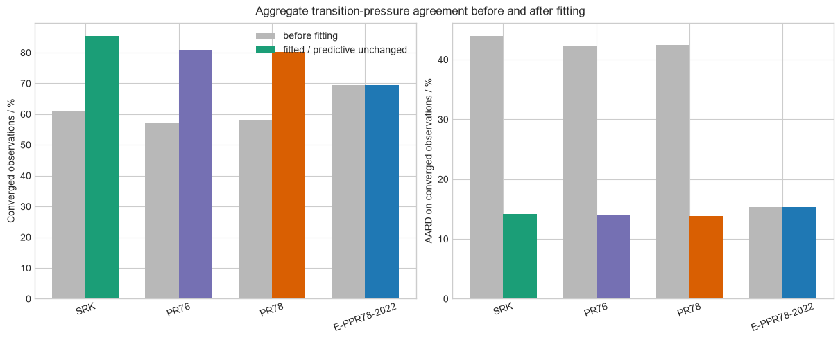
The fitted two-phase rows are calibration-domain agreement, while the fitted LL-VLL rows and every E-PPR78 row are validation evidence.

PyTorch execution and performance

The run used float64 on CPU with four PyTorch intra-operation threads. Transition states and grid states were grouped into compatible tensor batches. The trust-region invariant solver likewise evaluates independent residuals, gradients, and exact Hessian blocks in one tensor batch.

An isolated 40 by 40 PR78 phase-grid probe compared eager and compiled execution with identical phase counts, convergence flags, and fugacity residuals:

Mode	Cold / s	Warmed median / s
Eager	0.899	0.896
torch.compile	0.868	0.887

Compiled execution was not selected because the warmed improvement was below the declared 5% threshold.

Stage	Time / s
Unfitted observation-state evaluation	41.20
Unfitted/predictive phase grids	299.68
Three fits and sensitivity audits	123.56
Fitted observation-state evaluation	89.20
Fitted conventional phase grids	285.46
Sum	839.10

The phase grids remain the dominant cost. These timings include residual, phase-separation, material-balance, and boundary-refinement checks and are not comparable to a homogeneous-property call.

Limitations

Accepted observation-state branches satisfy a maximum dimensionless log-fugacity residual of \(10^{-7}\) and a minimum phase separation of \(2\times10^{-3}\). Grid cells use a \(10^{-8}\) fugacity threshold. Solver failure and phase collapse reduce coverage rather than being converted into numerical errors.

Calibration substantially improves conventional-cubic aggregate agreement, but L-LL branch coverage remains 27–41%. The full-rank local sensitivity matrices are not a proof of global identifiability, parameter uniqueness, or transfer outside the fitted systems. The broad phase-envelope domain includes fluid-model extrapolation, and pressure-limited L-L branches must not be read as closed curves.