Physical Phase Identification

Phase identification assigns a likely physical name—liquid or vapor—to an already selected homogeneous state. It answers a different question from equilibrium:

1. a root-selection operation supplies a molar volume \(V\);
2. a flash or stability calculation determines whether the state is an equilibrium phase; and
3. a phase-identification criterion labels that supplied state.

The label does not change the selected root, phase fraction, composition, or phase count. In particular, a small identification residual is not a stability test. For a flashed state, apply the criterion to each equilibrium phase composition after checking convergence, fugacity equality, and material balance.

torch-flash implements the five criteria compared by Bennett and Schmidt and the pressure-derivative parameter of Venkatarathnam and Oellrich. The implementation uses SI units and keeps the numerical criterion connected to the PyTorch computation graph.

Equilibrium-first grid algorithm

The grid procedure used before phase identification is a numerical continuation strategy, not a new thermodynamic equilibrium condition or a new phase-identification criterion. Reusing a previously converged equilibrium as an initial estimate is established practice in phase-envelope construction and compositional simulation. Michelsen (1980) used preceding envelope points to initialize continued solutions, then Michelsen (1982, Part II) formulated isothermal multiphase flashes as alternating stability and phase-split calculations with Gibbs-decreasing second-order refinement. Li and Firoozabadi likewise describe stability solutions or the previous simulation timestep as phase-split initial estimates. Current open-source flash interfaces also accept a prior flash result in place of separate phase-composition and volume guesses, for example the Clapeyron.jl flash API.

What is specific to torch-flash is the batched PyTorch realization, the selection of candidates from a two-dimensional grid, and the precise acceptance gates below. These are implementation choices within the established continuation and Gibbs-minimization framework; no novelty claim is made for the algorithm.

Independent flash at every state

Let grid cell \(k\) contain \((T_k,P_k,\mathbf{z}_k)\). The calculation first flashes every cell independently:

1. tangent-plane stability screens the feed;
2. unstable feeds enter a batched two-phase flash;
3. both returned phases are tested for further instability; and
4. failed or child-unstable states enter an up-to-three-phase Gibbs search.

The Gibbs search uses unconstrained component-allocation coordinates \(q_{pi}\):

\[ n_{pi} =z_i\frac{\exp(q_{pi})}{\sum_s\exp(q_{si})}, \qquad \beta_p=\sum_i n_{pi}, \qquad x_{pi}=\frac{n_{pi}}{\beta_p}. \]

Consequently,

\[ \sum_p n_{pi}=z_i, \qquad \sum_p\beta_p\mathbf{x}_p=\mathbf{z}, \]

so nonnegative component material balance is satisfied by construction. Autodiff supplies the Gibbs gradients. Distinct positive phases are polished with an equal-fugacity Newton solve before they can be installed.

Gibbs-gated boundary continuation

An independently converged grid can still contain adjacent cells that found different stationary Gibbs basins. A small fugacity residual proves that the installed split is stationary; it does not prove that no lower basin exists. For a two-dimensional grid, torch-flash therefore audits:

• lower-phase-count cells enclosed by higher-phase-count cells; and
• two-phase cells sharing an edge with an accepted three-phase cell.

For target cell \(t\), let \(s\) be the nearest accepted three-phase grid cell. Its component-allocation shares are

\[ a_{pi}^{(s)} = \frac{\beta_p^{(s)}x_{pi}^{(s)}} {\sum_q\beta_q^{(s)}x_{qi}^{(s)}}, \qquad q_{pi}^{(0)}=\ln a_{pi}^{(s)}. \]

The target feed is then repartitioned as

\[ n_{pi}^{(0)} = z_i^{(t)} \frac{\exp(q_{pi}^{(0)})} {\sum_q\exp(q_{qi}^{(0)})}. \]

This transfers only the source phase-allocation pattern and satisfies the target material balance exactly. The source compositions are not copied into the result. In particular, multicomponent three-phase compositions are not assumed constant along a pressure or composition row.

For three retained phases, the Newton variables are

\[ \mathbf{y} = \left( \ln\mathbf{K}_2,\, \ln\mathbf{K}_3,\, \ln\frac{\beta_2}{\beta_1},\, \ln\frac{\beta_3}{\beta_1} \right), \qquad K_{pi}=\frac{x_{pi}}{x_{1i}}. \]

The residual contains equal reduced chemical potentials,

\[ r_{pi}^{(\mu)} = \ln x_{pi}+\ln\phi_i(T,P,\mathbf{x}_p) - \ln x_{1i}-\ln\phi_i(T,P,\mathbf{x}_1) =0, \quad p\in\{2,3\}, \]

together with the two non-reference phase-normalization equations. PyTorch autodiff constructs the block-diagonal Newton Jacobian for the complete candidate batch.

A target replaces its installed state only if all of the following hold:

\[ \begin{aligned} r_f &= \max_{p>1,i}\left|r_{pi}^{(\mu)}\right| \leq\epsilon_f,\\ r_z &= \max_i\left| \sum_p\beta_px_{pi}-z_i \right| \leq\epsilon_z,\\ \min_p\beta_p &>\epsilon_\beta,\\ \min_{p<q}\lVert\mathbf{x}_p-\mathbf{x}_q\rVert_\infty &>\epsilon_x,\\ g_{\mathrm{candidate}} &< g_{\mathrm{installed}}-\epsilon_g. \end{aligned} \]

Here \(g=G/(RT)\). The continuation front advances until no new lower-Gibbs neighbor is accepted. A previously rejected cell is retried only when its nearest accepted three-phase seed changes. Unresolved candidates retain the independent multistart fallback; topology never overrides the thermodynamic gates.

For the float64 reference configuration, GridFlashOptions defaults to \(\epsilon_f=10^{-8}\), \(\epsilon_z=5\times10^{-11}\), \(\epsilon_\beta=10^{-4}\), \(\epsilon_x=2\times10^{-3}\), and \(\epsilon_g=2\times10^{-7}\). These values are numerical configuration, not phase-identification thresholds.

Identification and region assembly

Only after the equilibrium audit reaches this fixed point does identify_grid_phases evaluate a selected criterion on each retained equilibrium composition. The per-phase liquid/vapor labels and equilibrium phase count form the region code:

Equilibrium phases	Identified phases	Region
1	vapor	V
1	liquid	L
2	one vapor, one liquid	LV
2	two liquids	LL
3	any identified three-phase combination	three-phase
any	non-converged or unidentified	unavailable

The plotted map is this discrete region tensor. No image filter, contour interpolation, or post-hoc label smoothing is applied.

State and derivative convention

Let

\[ P=P(T,V,\mathbf{x}) \]

be an explicit pressure equation for the supplied homogeneous composition \(\mathbf{x}\). Composition is fixed in every derivative on this page. Define

\[ P_T=\left(\frac{\partial P}{\partial T}\right)_{V,\mathbf{x}}, \qquad P_V=\left(\frac{\partial P}{\partial V}\right)_{T,\mathbf{x}}, \]

and similarly \(P_{TT}\), \(P_{VT}\), and \(P_{VV}\). A mechanically stable homogeneous root satisfies

\[ V>0,\qquad P_V<0. \]

Along an isobar, \(P(T,V(T),\mathbf{x})\) is constant. Its first total derivative therefore gives

\[ 0=P_T+P_V\dot V, \qquad \dot V\equiv \left(\frac{\mathrm dV}{\mathrm dT}\right)_{P,\mathbf{x}} =-\frac{P_T}{P_V}. \]

Differentiating once more gives

\[ \ddot V\equiv \left(\frac{\mathrm d^2V}{\mathrm dT^2}\right)_{P,\mathbf{x}} =- \frac{ P_{TT}+2P_{VT}\dot V+P_{VV}\dot V^2 }{P_V}. \]

More generally, for any response \(F(T,V,\mathbf{x})\),

\[ \left(\frac{\mathrm dF}{\mathrm dT}\right)_{P,\mathbf{x}} =F_T+F_V\dot V =F_T-F_V\frac{P_T}{P_V}. \]

These identities are the common calculation behind the two response derivatives and the Venkatarathnam–Oellrich parameter.

Li pseudo-critical temperature

The pseudo-critical mixing rule was proposed by Li (1971). It forms volume-weighted component contributions

\[ w_i=x_iV_{c,i} \]

and estimates the phase pseudo-critical temperature as

\[ T_{\mathrm{pc}} =r_1 \frac{\sum_i w_iT_{c,i}}{\sum_i w_i} =r_1 \frac{\sum_i x_iV_{c,i}T_{c,i}} {\sum_i x_iV_{c,i}}. \]

Here \(T_{c,i}\) is in K, \(V_{c,i}\) is in \(\mathrm{m^3\,mol^{-1}}\), and \(r_1\) is a dimensionless tuning factor. torch-flash defaults to the value used in the comparison study, \(r_1=1\). The dimensionless score and exact decision are

\[ q_{\mathrm{Li}}=\frac{T}{T_{\mathrm{pc}}}, \qquad \begin{cases} q_{\mathrm{Li}}>1 &: \text{vapor},\\ q_{\mathrm{Li}}\leq1 &: \text{liquid}. \end{cases} \]

This criterion has no explicit pressure term. Pressure can still affect a post-flash label indirectly because the equilibrium phase composition \(\mathbf{x}\) changes with pressure. The method is unavailable if the model does not supply positive component critical volumes.

Pedersen volume-to-covolume rule

The defining source for this diagnostic is the reservoir-fluid monograph by Pedersen and Christensen, first published in 2006, and retained in section 6.6 of the current edition. It is a textbook criterion rather than a journal-paper proposal. The diagnostic compares the cubic-EoS volume with the mixture covolume \(b\):

\[ q_{V/b}=\frac{V_{\mathrm{EOS}}}{b(\mathbf{x})}. \]

For a conventional van der Waals one-fluid covolume, \(b(\mathbf{x})=\sum_i x_i b_i\). torch-flash uses the exact mixture covolume returned by the selected cubic model, so models with another supported covolume mixing rule retain that definition. The volume is obtained from the selected compressibility-factor root,

\[ V_{\mathrm{EOS}}=\frac{ZRT}{P}. \]

Cubic volume translations are deliberately excluded from this ratio: the criterion uses the volume associated with the repulsive cubic term and the same \(b\), not a translated property volume. With the recommended default \(r_2=1.75\),

\[ \begin{cases} V_{\mathrm{EOS}}/b>r_2 &: \text{vapor},\\ V_{\mathrm{EOS}}/b\leq r_2 &: \text{liquid}. \end{cases} \]

The public threshold option exposes \(r_2\), so a non-default value is a scientific model choice and should be recorded with the result. See Pedersen, Christensen, and Shaikh, section 6.6, for the cubic-EoS rule used by default.

Perschke negative-flash residual

The phase-label shortcut is attributed to Perschke's 1988 dissertation. It uses the negative-flash extension formalized by Whitson and Michelsen (1989) and Wilson's 1968 equilibrium-ratio estimate. For the supplied composition, define the two-phase Rachford–Rice function

\[ G(\beta)= \sum_i \frac{x_i(K_i-1)} {1+\beta(K_i-1)}. \]

For positive \(K_i\) and admissible denominators,

\[ \frac{\mathrm dG}{\mathrm d\beta} =- \sum_i \frac{x_i(K_i-1)^2} {\left[1+\beta(K_i-1)\right]^2} \leq0, \]

so \(G\) is monotone non-increasing. Perschke's shortcut evaluates the function only at \(\beta=0.5\):

\[ G(0.5)= \sum_i \frac{x_i(K_i^{W}-1)} {1+0.5(K_i^{W}-1)}. \]

The Wilson estimates used outside as well as inside the two-phase region are

\[ K_i^{W} =\frac{P_{c,i}}{P} \exp\left[ 5.373(1+\omega_i) \left(1-\frac{T_{c,i}}{T}\right) \right]. \]

Because \(G\) decreases with \(\beta\), a positive \(G(0.5)\) places its root above \(0.5\), while a negative value places it below \(0.5\). For a stable homogeneous state, the negative-flash root is outside the physical interval \((0,1)\), giving the \(>1\) vapor and \(<0\) liquid interpretation described by Perschke. The implemented shortcut is

\[ \begin{cases} G(0.5)>0 &: \text{vapor},\\ G(0.5)\leq0 &: \text{liquid}. \end{cases} \]

This is a homogeneous-state diagnostic constructed from an estimated \(K\)-value correlation. It does not execute a negative flash, establish stability, or replace the converged equilibrium ratios of a flash.

Isothermal-compressibility derivative

The temperature-derivative criterion was proposed by Pasad and Venkatarathnam (1999). The isothermal compressibility is

\[ \kappa_T =-\frac{1}{V} \left(\frac{\partial V}{\partial P}\right)_{T,\mathbf{x}} =-\frac{1}{VP_V}, \]

with units \(\mathrm{Pa^{-1}}\). Applying the constant-pressure chain rule gives

\[ \left(\frac{\partial\kappa_T}{\partial T}\right)_{P,\mathbf{x}} = \frac{ VP_{VT} - \left(P_V+VP_{VV}\right)P_T/P_V }{ \left(VP_V\right)^2 }. \]

The same quantity can be evaluated without expanding the fraction:

\[ \left(\frac{\partial\kappa_T}{\partial T}\right)_{P,\mathbf{x}} = \left(\frac{\partial\kappa_T}{\partial T}\right)_{V,\mathbf{x}} + \left(\frac{\partial\kappa_T}{\partial V}\right)_{T,\mathbf{x}} \dot V. \]

torch-flash uses this second form with nested forward-mode torch.func.jvp evaluations. It avoids finite-difference steps and preserves the graph through \(T\), \(P\), composition, the selected molar volume, and trainable model parameters. The criterion has units \(\mathrm{Pa^{-1}\,K^{-1}}\):

\[ \begin{cases} (\partial\kappa_T/\partial T)_P>0 &: \text{liquid or liquid-like},\\ (\partial\kappa_T/\partial T)_P\leq0 &: \text{vapor-like}. \end{cases} \]

Thermal-expansion derivative

The thermal-expansion criterion was proposed by Bennett and Schmidt (2017). The isobaric thermal-expansion coefficient is

\[ \alpha_P =\frac{1}{V} \left(\frac{\partial V}{\partial T}\right)_{P,\mathbf{x}} =\frac{\dot V}{V} =-\frac{P_T}{VP_V}, \]

with units \(\mathrm{K^{-1}}\). Its constant-pressure temperature derivative can be written either as a response chain rule,

\[ \left(\frac{\partial\alpha_P}{\partial T}\right)_{P,\mathbf{x}} = \left(\frac{\partial\alpha_P}{\partial T}\right)_{V,\mathbf{x}} + \left(\frac{\partial\alpha_P}{\partial V}\right)_{T,\mathbf{x}} \dot V, \]

or in terms of the first and second isobaric volume derivatives:

\[ \left(\frac{\partial\alpha_P}{\partial T}\right)_{P,\mathbf{x}} =\frac{\ddot V}{V} -\left(\frac{\dot V}{V}\right)^2. \]

Substituting the pressure derivatives from the common calculation gives

\[ \left(\frac{\partial\alpha_P}{\partial T}\right)_{P,\mathbf{x}} =- \frac{ P_{TT}+2P_{VT}\dot V+P_{VV}\dot V^2 }{VP_V} -\alpha_P^2. \]

torch-flash again evaluates the response chain rule with nested forward-mode JVPs. The score has units \(\mathrm{K^{-2}}\), and Bennett's decision is

\[ \begin{cases} (\partial\alpha_P/\partial T)_P>0 &: \text{liquid or liquid-like},\\ (\partial\alpha_P/\partial T)_P\leq0 &: \text{vapor-like}. \end{cases} \]

Venkatarathnam–Oellrich phase-identification parameter

The dimensionless parameter was proposed by Venkatarathnam and Oellrich (2011):

\[ \Pi =V\left( \frac{P_{VT}}{P_T} - \frac{P_{VV}}{P_V} \right). \]

The direct decision is

\[ \begin{cases} \Pi>1 &: \text{liquid or liquid-like},\\ \Pi\leq1 &: \text{vapor-like}. \end{cases} \]

Its connection to the compressibility criterion follows immediately by factoring the expanded derivative:

\[ \left(\frac{\partial\kappa_T}{\partial T}\right)_{P,\mathbf{x}} = \frac{P_T}{V^2P_V^2}(\Pi-1). \]

Therefore, when \(P_T>0\), the two criteria have exactly the same sign and decision boundary. If \(P_T<0\), the sign relation reverses; if \(P_T=0\), \(\Pi\) is undefined. The published criterion assumes the conventional positive-\(P_T\) states for which the equivalence is used.

The implementation evaluates \(P_T\), \(P_V\), \(P_{VT}\), and \(P_{VV}\) with nested torch.func.jvp calls. For a leading state batch, every pressure output depends only on the corresponding \(T,V,\mathbf{x}\) input. Directional derivatives along all-one \(T\) or \(V\) tangents therefore recover the independent Jacobian diagonals without constructing a dense batch Jacobian.

The calculation rejects \(P_V\geq0\) as mechanically unstable. It also guards the two denominators using

\[ |P_T|\leq\tau|P/T|, \qquad |P_V|\leq\tau|P/V|, \]

where \(\tau=\sqrt{\epsilon_{\mathrm{machine}}}\) by default. Through identify_phase, a singular or mechanically unstable evaluation becomes an ambiguous unknown, not an infinite score.

The local \(\Pi\) rule can identify some far-superheated states as liquid-like after a high-temperature inversion. The source paper gives an additional remote-temperature correction and notes that it is unnecessary when the method labels saturated split phases after a converged flash. torch-flash implements the local parameter and does not perform that remote temperature search. For arbitrary superheated homogeneous states, interpret the result as a local liquid-like/vapor-like diagnostic.

Decision and ambiguity summary

Public method name	Stored criterion	Threshold	Exact vapor decision
li-pseudo-critical-temperature	\(T/T_{\mathrm{pc}}\)	\(1\)	\(T/T_{\mathrm{pc}}>1\)
pedersen-volume-to-covolume	\(V_{\mathrm{EOS}}/b\)	\(1.75\) by default	\(V_{\mathrm{EOS}}/b>1.75\)
perschke-negative-flash	\(G(0.5)\)	\(0\)	\(G(0.5)>0\)
pasad-isothermal-compressibility-derivative	\((\partial\kappa_T/\partial T)_P\)	\(0\)	criterion \(\leq0\)
bennett-thermal-expansion-derivative	\((\partial\alpha_P/\partial T)_P\)	\(0\)	criterion \(\leq0\)
venkatarathnam-oellrich-phase-identification-parameter	\(\Pi\)	\(1\)	\(\Pi\leq1\)

The exact inequality always determines kind. Separately, ambiguous=True marks a score close to its separator. With relative tolerance \(r\), which defaults to \(0.05\):

• Li and Pedersen use a symmetric log-ratio band, \(\left|\ln(q/q_*)\right|\leq\ln(1+r)\);
• Perschke scales the band by the sum of absolute Rachford–Rice terms;
• each response derivative scales the band by the sum of the absolute constant-pressure chain-rule terms; and
• the \(\Pi\) method uses \(|\Pi-1|\leq r\).

This flag exposes a numerically or physically weak label without silently changing the exact literature decision.

Minimal API example

The public API accepts one scalar \(T,P,\mathbf{x}\) state. The phase argument selects the EoS root to evaluate; it is not the returned physical identity:

import torch

from torch_flash import (
    ChemicalState,
    PhaseIdentificationCriterion,
    component_set,
    configure,
    identify_phase,
    peng_robinson_1978,
)

configure(dtype=torch.float64, device="cpu", num_threads=1)
model = peng_robinson_1978(component_set(("methane", "n_butane")))
temperature = torch.tensor(250.0, requires_grad=True)
state = ChemicalState(
    temperature=temperature,
    pressure=torch.tensor(10.0e6),
    composition=torch.tensor([0.5, 0.5]),
)

methods: tuple[PhaseIdentificationCriterion, ...] = (
    "li-pseudo-critical-temperature",
    "pedersen-volume-to-covolume",
    "perschke-negative-flash",
    "pasad-isothermal-compressibility-derivative",
    "bennett-thermal-expansion-derivative",
    "venkatarathnam-oellrich-phase-identification-parameter",
)
results = {
    method: identify_phase(model, state, phase="stable", method=method)
    for method in methods
}

for method, result in results.items():
    value = None if result.criterion_value is None else result.criterion_value.detach()
    print(method, result.kind, value, result.ambiguous)

# Criterion tensors retain their graph; string labels do not.
pip = results["venkatarathnam-oellrich-phase-identification-parameter"]
d_pip_d_temperature = torch.autograd.grad(pip.criterion_value, temperature)[0]

At this state all six methods return an unambiguous liquid label. Always check criterion_value is not None before differentiating a method that can be unavailable. For an already flashed grid, use identify_grid_phases; the batched grid guide shows the complete equilibrium-first workflow.

Comparison on the North Ward Estes injection case

The following project-generated verification result uses the paper's \(500\times500\) grid resolution to resolve the narrow three-phase band. It uses PR78 at \(301.48\ \mathrm{K}\), a 95 mol% CO2 + 5 mol% methane injection gas, and the seven-component North Ward Estes oil data reported by Li and Firoozabadi. The plotted axes are injected-gas mole fraction and pressure from 50 to 200 bar.

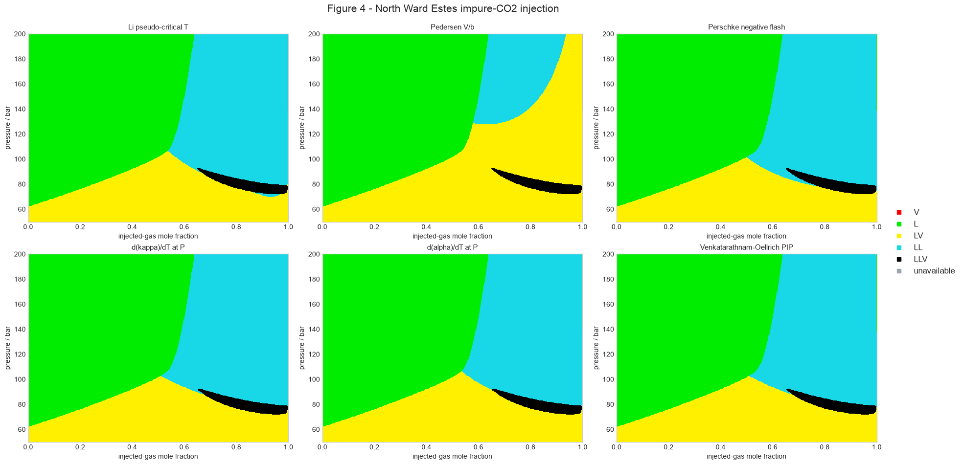
The LLV boundary is obtained from the equilibrium calculation, not from image processing. Independent multistart flashes can occasionally converge to a two-phase stationary point while a nearby three-phase Gibbs basin is lower; small fugacity and material-balance residuals establish stationarity and closure, but do not by themselves prove that the lowest basin was found. The grid solver therefore uses each accepted three-phase state as a local continuation seed for adjacent two-phase cells and repeats the target-state equal-fugacity solve. The candidate is installed only if it lowers the existing Gibbs energy and passes the original residual tolerances.

Every one of the 250,000 cells was flashed before applying each diagnostic to the returned equilibrium phase compositions. All cells converged; the maximum log-fugacity residual was \(9.9998\times10^{-9}\), the maximum material-balance residual was \(3.4839\times10^{-13}\), and 4,066 cells were three-phase. The grid flash independently audited 1,217 distinct enclosed or three-phase-boundary cells and accepted 850 lower-Gibbs replacements. Neighboring equilibria were used only as initial guesses for target-state autodiff-Newton solves; no plotted label was smoothed or copied. No horizontally or vertically bracketed two-phase cell remained. The published inputs omit component critical volumes, so PR-consistent values were derived only for Li's labeling rule; they do not enter the equilibrium flash.

The result is particularly informative because the methods agree on the broad equilibrium topology but not on every physical label. Across valid cells, the mean pairwise region-code agreement was 93.26%, the least-agreeing pair was 80.27%, and at least one method differed in 19.83% of cells. Pedersen's rule produces the visibly largest injection-rich LV region. The \(\Pi\) and \((\partial\kappa_T/\partial T)_P\) maps agree in all 250,000 cells, which independently checks their algebraic equivalence for these mechanically stable states.

The recorded float64 CPU wall times below are complete standalone method passes over the same flashed phases; practical use normally selects one row, not all six. The comparison ran with one PyTorch intra-op thread on the recorded Apple-silicon host, so timings characterize this saved study rather than other hardware.

Method	Identification wall time
Li pseudo-critical temperature	46.826 ms
Pedersen \(V/b\)	464.864 ms
Perschke negative flash	98.476 ms
Venkatarathnam–Oellrich \(\Pi\)	3.735 s
Bennett \((\partial\alpha_P/\partial T)_P\)	9.250 s
Pasad/Venkatarathnam \((\partial\kappa_T/\partial T)_P\)	8.687 s

This is verification of the implemented diagnostics and equilibrium workflow, not validation against experimental phase labels or a pixel-wise reconstruction of the paper's nominal \(500\times500\) raster. The complete reproducible calculation, residual audits, timing environment, and all five paper cases are in 29_bennett_phase_identification_methods. The documentation profile sets TORCH_FLASH_PHASE_ID_NWE_GRID_POINTS=500; the other four saved cases retain their default \(100\times100\) grids.

References

1. C. C. Li, “Critical Temperature Estimation for Simple Mixtures,” Canadian Journal of Chemical Engineering 49(5), 709–710 (1971). doi:10.1002/cjce.5450490529.
2. K. S. Pedersen and P. L. Christensen, Phase Behavior of Petroleum Reservoir Fluids, 1st ed., CRC Press (2006). doi:10.1201/9781420018257.
3. K. S. Pedersen, P. L. Christensen, and J. A. Shaikh, Phase Behavior of Petroleum Reservoir Fluids, 3rd ed., CRC Press (2024), section 6.6. doi:10.1201/9780429457418.
4. D. R. Perschke, “Development and Application of an Equation of State Compositional Simulator,” PhD dissertation, The University of Texas at Austin (1988).
5. D. R. Perschke, G. A. Pope, and K. Sepehrnoori, “Phase Identification During Compositional Simulation,” paper SPE-19442-MS, 64th SPE Annual Technical Conference and Exhibition, San Antonio, Texas (1989). doi:10.2118/19442-MS.
6. C. H. Whitson and M. L. Michelsen, “The Negative Flash,” Fluid Phase Equilibria 53, 51–71 (1989). doi:10.1016/0378-3812(89)80072-X.
7. G. A. Wilson, “A Modified Redlich–Kwong Equation of State Applicable to General Physical Data Calculations,” paper 15C, 65th AIChE National Meeting, Cleveland, Ohio (1968).
8. G. V. Pasad and G. Venkatarathnam, “A Method for Avoiding Trivial Roots in Isothermal Flash Calculations Using Cubic Equations of State,” Industrial & Engineering Chemistry Research 38(9), 3530–3534 (1999). doi:10.1021/ie980661t.
9. G. Venkatarathnam and L. R. Oellrich, “Identification of the Phase of a Fluid Using Partial Derivatives of Pressure, Volume and Temperature without Reference to Saturation Properties: Applications in Phase Equilibria Calculations,” Fluid Phase Equilibria 301, 225–233 (2011). doi:10.1016/j.fluid.2010.12.001.
10. J. Bennett and Z. Schmidt, “Comparison of Phase Identification Methods Used in Petroleum Reservoir Simulation,” Energy & Fuels 31, 3370–3379 (2017). doi:10.1021/acs.energyfuels.6b02316.
11. Z. Li and A. Firoozabadi, “General Strategy for Stability Testing and Phase-Split Calculation in Two and Three Phases,” SPE Journal 17(4), 1096–1107 (2012). doi:10.2118/129844-PA.
12. M. L. Michelsen, “Calculation of Phase Envelopes and Critical Points for Multicomponent Mixtures,” Fluid Phase Equilibria 4, 1–10 (1980). doi:10.1016/0378-3812(80)80001-X.
13. M. L. Michelsen, “The Isothermal Flash Problem. Part I. Stability,” Fluid Phase Equilibria 9, 1–19 (1982). doi:10.1016/0378-3812(82)85001-2.
14. M. L. Michelsen, “The Isothermal Flash Problem. Part II. Phase-Split Calculation,” Fluid Phase Equilibria 9, 21–40 (1982). doi:10.1016/0378-3812(82)85002-4.
15. Clapeyron.jl contributors, “Multiphase Properties: Flash Methods,” Clapeyron.jl documentation. Flash API.